NeurIPS 2026

FLINT: Coupling Proximal Initialization
and Bounded Stochasticity for
Flow-Matching Inverse Problems

Junseo Bang1, Daewon Choi2, Dong Ju Mun1, Se Young Chun1,2,3†

1Dept. of ECE   2IPAI   3INMC & AIIS, Seoul National University

†Corresponding author

Initialize close enough, sample carefully to keep it. FLINT first moves the initial noise near one that the model maps to an image consistent with the measurement, then samples with little noise while the image takes shape. The result: state-of-the-art perceptual quality and competitive distortion metrics, at a lower sampling cost than the flow-matching baselines.
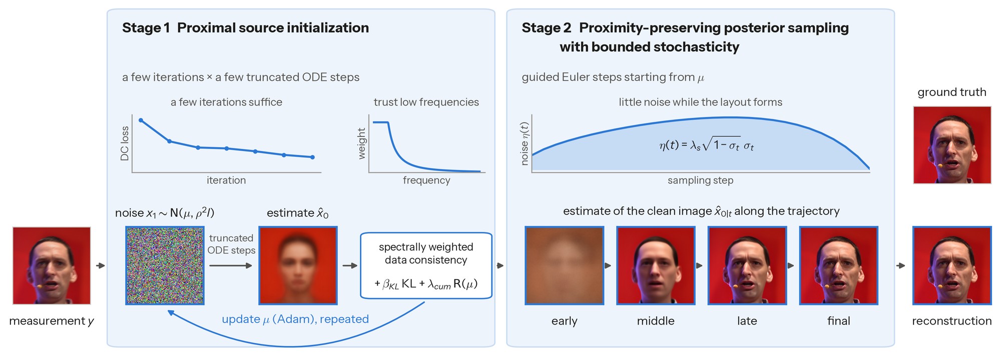
FLINT pipeline: a measurement, Stage 1 optimizing the initial noise in a few iterations, Stage 2 sampling with a bell-shaped noise schedule, and the reconstruction next to the ground truth.

Abstract

Flow matching models have emerged as a dominant paradigm for generative posterior sampling in imaging inverse problems. Existing solvers follow two distinct lines of work: trajectory-space methods, which refine sampling dynamics from random initial noise, and source-space methods, which optimize the initial noise itself. While most prior work treats these as independent design choices, we show that they are inherently coupled. We derive a unified stability bound that links initialization proximity and cumulative sampling stochasticity through a multiplicative envelope, complemented by two empirical observations. First, we identify a sufficiency regime in which a moderately optimized proximal source initialization is enough to attain the performance plateau, rendering exhaustive source-space optimization unnecessary. Second, this initial advantage is fragile: it is eroded by excessive stochasticity accumulation during guided sampling, necessitating a mechanism that bounds the cumulative noise injection. These findings motivate FLINT, a two-stage framework that operationalizes this coupling. FLINT establishes a high-fidelity starting point via a manifold-constrained proximal objective in only a few iterations, then performs guided sampling under a bounded stochasticity schedule that helps prevent erasure of the initialization advantage. Across diverse inverse problems, FLINT delivers state of the art perceptual quality and competitive distortion metrics while maintaining superior computational efficiency.

Initialization and stochasticity are coupled

Most solvers either steer the sampling trajectory from random noise or optimize the initial noise itself, and the two are usually treated as separate design choices.

Five panels on stacked noise-level manifolds from M1 at the top to M0 at the bottom, with the measurement subspace y = Ax as a green line. Trajectory-space methods: (a) DPS and FlowChef start from random noise and alternate a generative step with a measurement-guided correction on every noisy state; (b) FlowDPS and Flower jump to the clean estimate, correct it and re-noise to the next level. Source-space methods: (c) DMPlug and D-Flow run many MAP iterations on the initial noise, then one deterministic flow to x0; (d) N-HMC and D-Flow SGLD sample the initial noise with Hamiltonian or Langevin dynamics instead. (e) FLINT: a short measurement-guided move from the random start to a proximal start, then a guided trajectory inside a narrow band of bounded stochasticity that ends where M0 meets the measurement subspace.
Where FLINT sits. Trajectory-space methods start from random noise and steer every step: (a) a likelihood correction on each noisy state xt, or (b) a correction on the clean estimate x̂0|t followed by re-noising to the next noise level. Source-space methods act on the initial noise through the deterministic flow map x0 = Φ(x1): (c) MAP optimization, or (d) posterior sampling of x1 with Hamiltonian or Langevin dynamics. (e) FLINT couples a proximal source initialization x̃1, reached in a few iterations, with bounded stochasticity during guided sampling, to help the trajectory keep the advantage of the initialization.

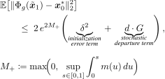
Our analysis puts them in one bound. Take a reference noise x1* that is typical under the prior and consistent with the measurement, and let x0* be the output of the same guided sampler run from x1* with its injected noise switched off. A start x̃1 within distance δ of x1* then gives a sample Φg(x̃1) that obeys (Proposition 3.1)

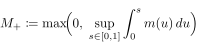
E of the squared distance between Phi_g of x-tilde_1 and x_0-star is at most 2 e to the 2 M-plus, times delta squared, the initialization error term, plus d times G, the stochastic departure term,with M-plus defined as the maximum of 0 and the supremum over s in [0, 1] of the integral from 0 to s of m(u) du.E of the squared distance between Phi_g of x-tilde_1 and x_0-star is at most 2 e to the 2 M-plus, times delta squared, the initialization error term, plus d times G, the stochastic departure term, with M-plus defined as the maximum of 0 and the supremum over s in [0, 1] of the integral from 0 to s of m(u) du.

where d is the dimension, G the stochasticity accumulated during sampling, and m(t) bounds how fast nearby trajectories separate. The two terms add up under a common prefactor. This motivates two design choices.

A nearby start is enough

Once δ² ≪ d·G, pushing δ further barely lowers the bound, and empirically quality plateaus long before exact inversion (the sufficiency regime below).

↳ Exhaustive source-space optimization buys little.

Too much noise erases it

A large G raises the bound for every start, however close: for a fixed M+ the bound grows with G. The noise injected during sampling has to stay limited.

↳ A good start is wasted if the sampler randomizes it away.

How the starting point and the injected noise affect quality. a: quarter-circle diagram of the spherical interpolation from the exact inversion of the ground truth (C0 = 0) through the proximal start (C0 = 0.4) to random noise (C0 = pi/2). b, c: PSNR and LPIPS against C0 for four levels of the cumulative stochasticity G; all curves stay flat up to C0 = 0.4, and larger G lowers and flattens them. d: posterior samples, zooms and unconditional samples from the three starts; the random start loses hair detail and its unconditional sample is a different person.
How close the start has to be, and how much injected noise erases the advantage (FlowDPS, Gaussian deblurring, 100 FFHQ images). (a) Every start lies on a spherical interpolation x1(C0) = [sin(θ − C0) x1* + sin C0 ε] / sin θ between x1*, the ground truth inverted by the unconditional flow ODE (exact inversion), and a Gaussian noise ε; θ ≈ π/2 is the angle between them. (b, c) PSNR and LPIPS of the posterior samples, for four levels of the cumulative stochasticity G = ∫01 gt2 dt (G = 0: deterministic sampling). In this setup quality stays flat up to C0 ≈ 0.4, the sufficiency regime, while a larger G lowers every curve and shrinks the gap between a close start and the random one. (d) Posterior samples at G = 0.008 next to the unconditional sample generated from the same start without the measurement.

Method

A few cheap iterations to start close, then sampling that keeps the injected noise small while the layout forms.

Stage 1 Proximal source initialization

A few Adam iterations on μ, the mean of a Gaussian variational distribution over the initial noise. Each iteration forms a clean estimate by truncated sampling, scores it with a Wiener-weighted data-consistency loss that trusts low frequencies plus KL and cumulant terms that keep μ Gaussian-like, and backpropagates through the first step only via the SDO shortcut.

Stage 2 Proximity-preserving posterior sampling with bounded stochasticity

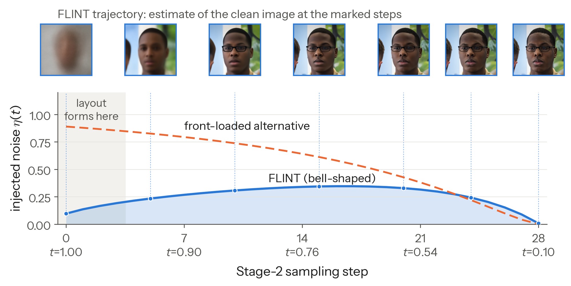
Guided sampling from μ: estimate the clean image, correct it toward the measurement, re-noise with η(t) = λs√(1−σt)·σt, which is small at t ≈ 1 and at t ≈ 0.
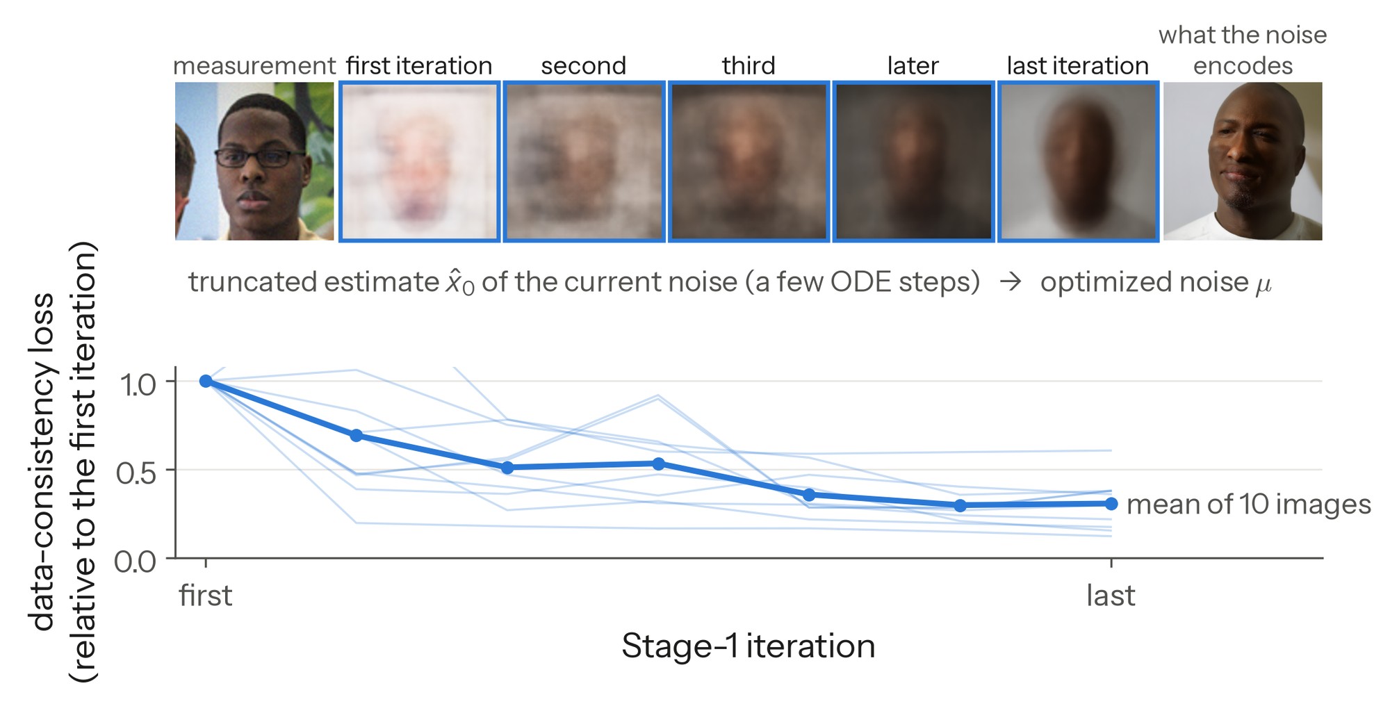
Stage-1 estimates and loss curve over the iterations.
The data-consistency loss plateaus within a few iterations.
Injected noise per step for the bell-shaped and the front-loaded schedules.
Little noise while the layout forms, more where detail is refined: the schedule protects the proximal start.
Sampling trajectories of FLINT and three baselines. a: estimates of the clean image at t = 0.9, 0.8, 0.6, 0.4 and 0 for FlowChef, FlowDPS, Flower and FLINT on one face; FLINT already shows the face and its hair at t = 0.9, while the baselines are blurred or distorted. b: PSNR and LPIPS of the estimate against the timestep for the four methods; FLINT (Ours) is highest in PSNR and lowest in LPIPS from early on to t = 0.
Sampling trajectories of FLINT and three baselines. (a) Tweedie estimate of the clean image along the sampling trajectory for FlowChef, FlowDPS, Flower and FLINT. (b) PSNR and LPIPS of that estimate along the trajectory (Ours = FLINT). FLINT enters the measurement-consistent region earlier than the three: its estimate already reflects the coarse structure of the reconstruction at t = 0.9 and then only refines detail, while the baselines are still forming the layout through much of the trajectory, and it keeps the highest quality of the four down to t = 0.

Results

Quantitative comparison

1,000 FFHQ and 800 DIV2K images at 768×768, measurement noise σy = 0.03, 50 NFEs for every method, all on Stable Diffusion 3.5-Medium.
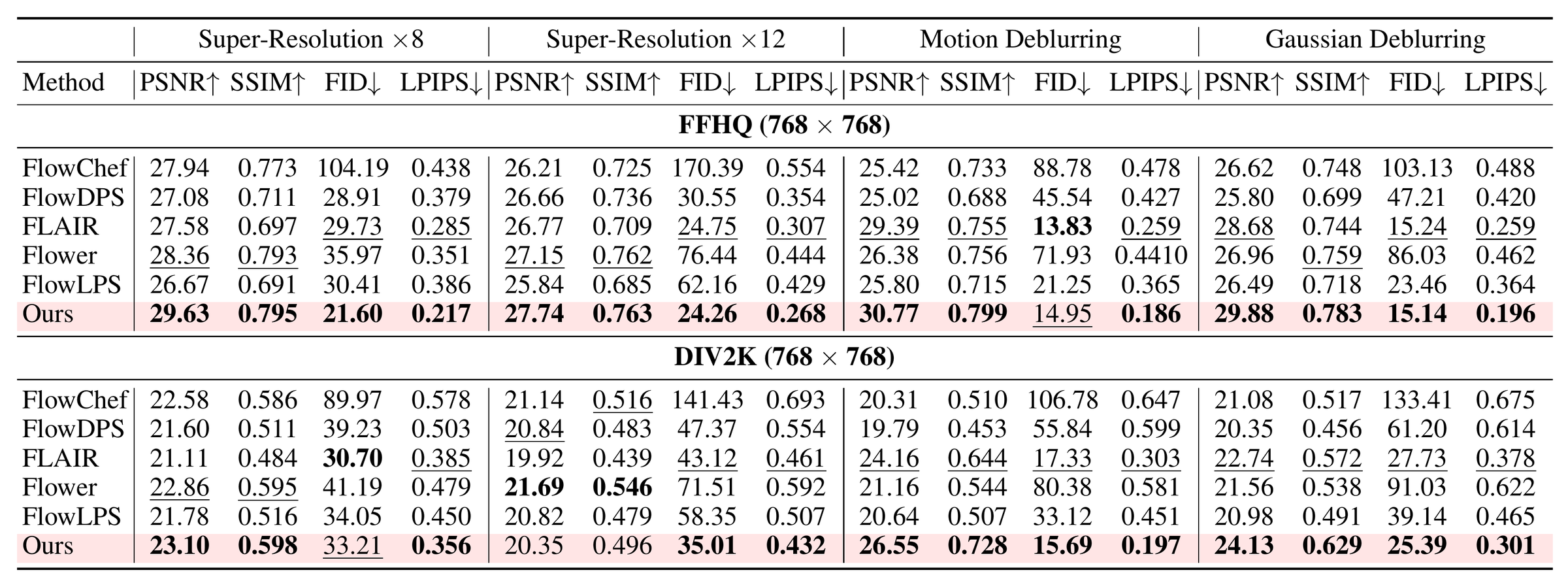
PSNR, SSIM, FID and LPIPS of FlowChef, FlowDPS, FLAIR, Flower, FlowLPS and FLINT for super-resolution x8 and x12, motion deblurring and Gaussian deblurring on FFHQ and DIV2K at 768 x 768.
Averages over 1,000 FFHQ and 800 DIV2K images with 50 NFEs and Gaussian noise σy = 0.03.

Computational cost vs. performance

Cost and quality: PSNR and LPIPS against sampling time in seconds for super-resolution x8 and Gaussian deblurring on FFHQ; FLINT at 25, 30, 40 and 50 NFEs lies above and left of FlowChef, FlowDPS, FLAIR, Flower and FlowLPS.
PSNR and LPIPS against sampling time (s) on FFHQ for super-resolution ×8 and Gaussian deblurring; the number after FLINT is its NFE count. With 30 NFEs FLINT already surpasses nearly all 50-NFE baselines on PSNR and LPIPS.

BibTeX

@inproceedings{bang2026flint,
  title     = {{FLINT}: Coupling Proximal Initialization and Bounded Stochasticity for Flow-Matching Inverse Problems},
  author    = {Bang, Junseo and Choi, Daewon and Mun, Dong Ju and Chun, Se Young},
  booktitle = {Advances in Neural Information Processing Systems},
  year      = {2026}
}